ARMA ARCH Simulation

Methodology

Manual Simulation

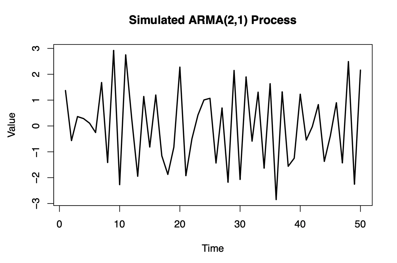
An ARMA(2,1) process of length 50 was simulated with parameters:

$$\phi_1 = -0.5, \phi_2 = 0.1, \theta_1 = 0.3$$

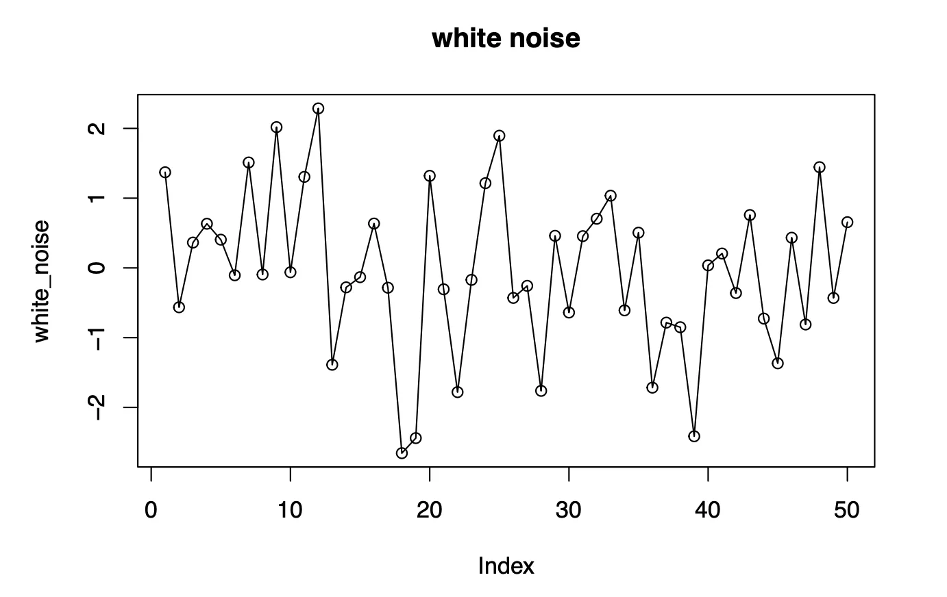
A burn-in period of 3 iterations was used to stabilize the process and a pre-specified white-noise series was provided to ensure reproducibility.

The process was computed iteratively using the ARMA(2,1) relationship:

$$Y_t = \phi_1 Y_{t-1} + \phi_2 Y_{t-2} + \epsilon_t - \theta_1 \epsilon_{t-1}$$

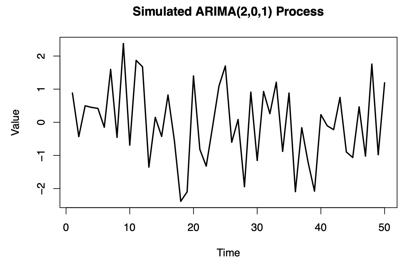
R’s arima.sim Function

The same ARMA(2,1) process was generated using the arima.sim function. The burn-in values were set manually to match the initial conditions from step 1. This approach served to validate the manually computed series.

Autocorrelation Analysis

Theoretical autocorrelation was computed using the ARMAacf function. Sample autocorrelation functions (ACFs) were calculated for both manually simulated and arima.sim series. Differences between theoretical and sample ACFs were analyzed.

Interpretation

Essentially, we are comparing the theoretical expectations with what we observed in the simulated data. In both cases, theoretical and sample ACFs, we have the autocorrelation values at various lags. Based on the general patterns, we see that the autocorrelation values in the theoretical ACF tend to be larger in magnitude compared to those in the sample ACF, especially at higher lags. The signs of the autocorrelation values alternate more frequently in theoretical ACF compared to sample ACF, where they appear to be more consistent. The autocorrelation values from sample ACF deviate more from the theoretical expectations to a greater extent compared to those in theoretical ACF. This could suggest that the model used in sample ACF might not fully capture the underlying process, leading to discrepancies between the simulated and theoretical results.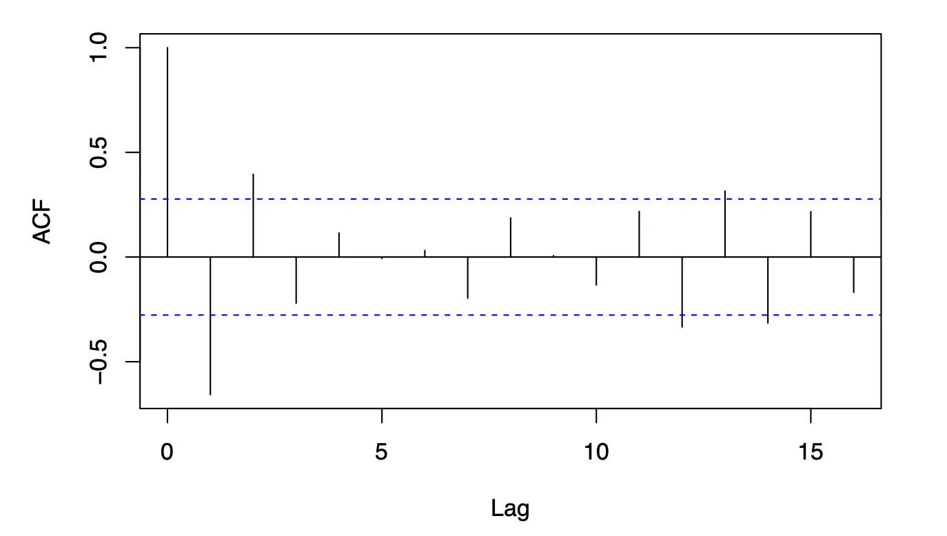

Theoretical autocorrelation

Sample ACF

Extended Realizations

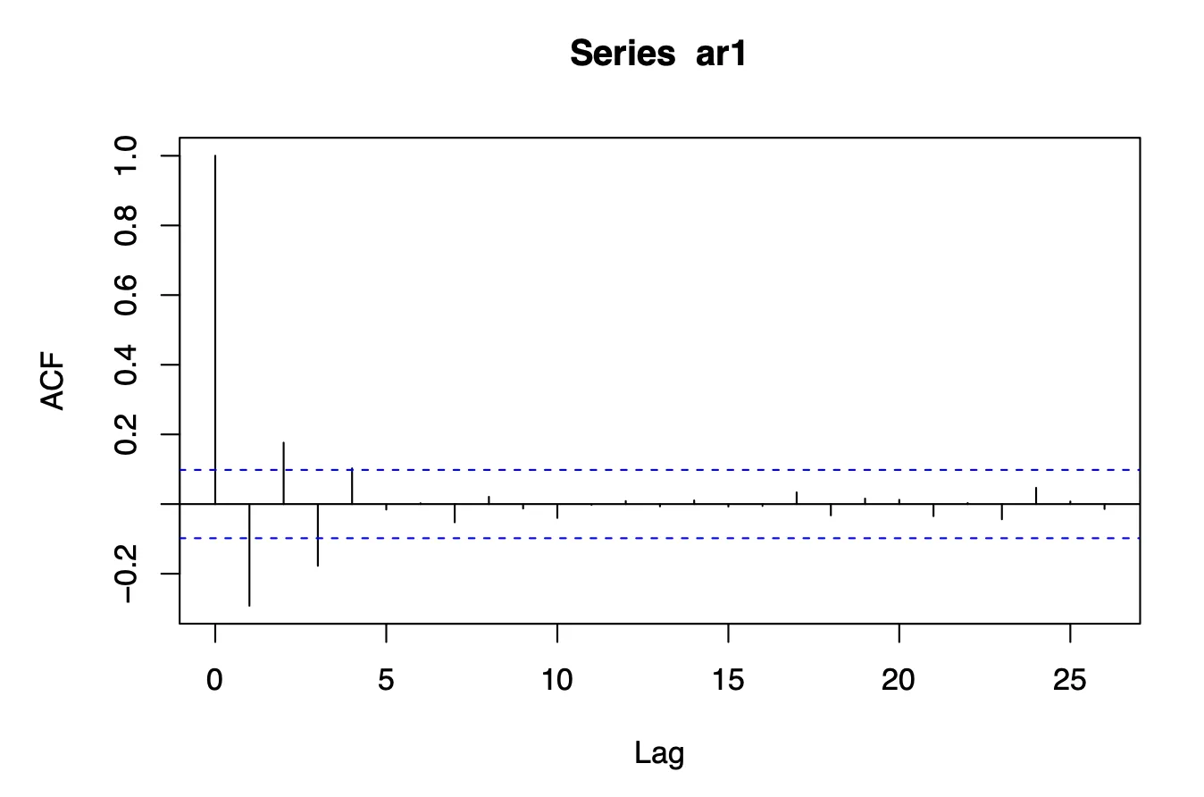
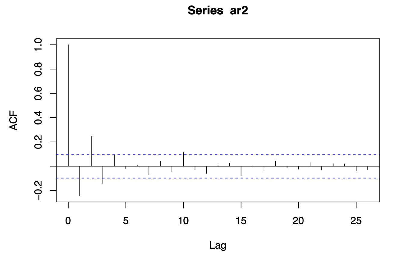
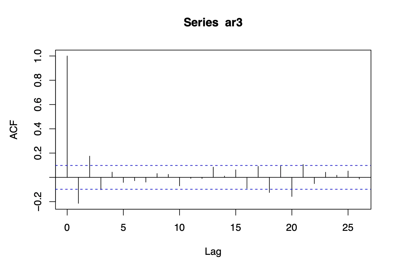
Four independent realizations of length 400 were generated using arima.sim. Sample ACFs were plotted for each realization, and their variability was discussed.

Results

Manual vs. arima.sim Comparison

The two methods produced series with similar trends but slight deviations due to differences in implementation. Sample ACFs showed minor discrepancies, especially at higher lags, emphasizing the stochastic nature of the white-noise component.

Theoretical vs. Sample ACFs

Theoretical ACFs matched closely at lower lags but deviated slightly as the lag increased, particularly for the arima.sim series. Alternating signs of ACF values aligned with the negative and positive feedback introduced by $\phi_1$ and $\phi_2$.

Extended Realizations

All four realizations displayed consistent patterns in ACFs, with minor variations due to random white noise. Peaks at initial lags confirmed significant short-term autocorrelation.

ARCH(1) Process Simulation and Analysis

Methodology

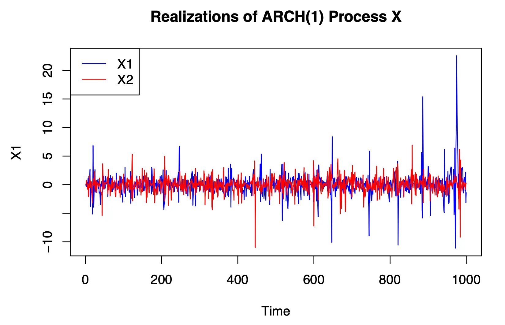
Simulation of ARCH(1) Process

An ARCH(1) process of length 1,000 was simulated using the model:

$$X_t = \epsilon_t \sqrt{\alpha + X_{t-1}^2}$$

where $\alpha = 0.5$, and $\epsilon_t$ is standard normal noise.

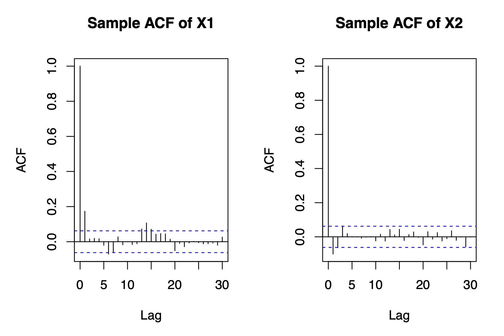
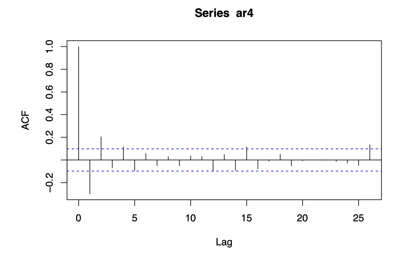
ACF Analysis

Sample ACFs of two realizations were computed and plotted. Weak white noise characteristics (stationarity and uncorrelated structure) were evaluated.

Ljung-Box Test

Applied the Ljung-Box test to detect autocorrelation in the realizations. Results supported the weak white noise properties of the ARCH(1) process.

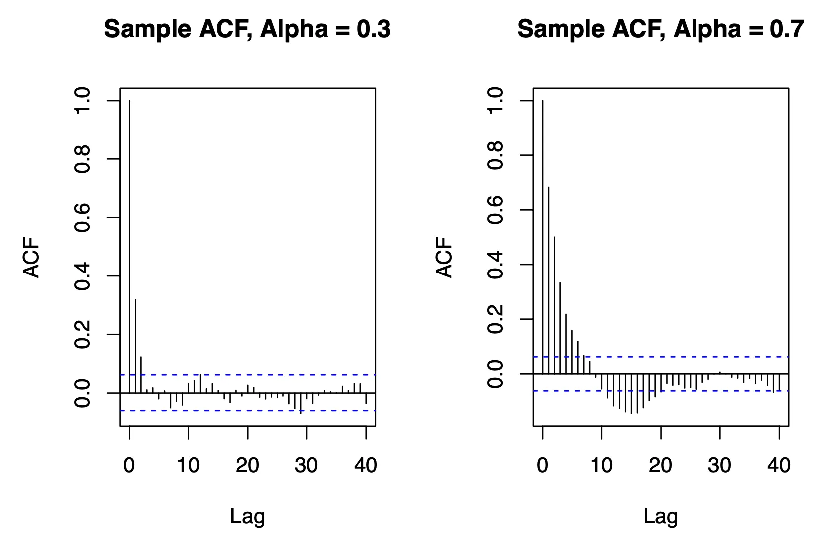
Influence of Parameter $\alpha$

Two realizations were simulated with $\alpha = 0.3$ and $\alpha = 0.7$. Sample ACFs were compared to study the influence of $\alpha$ on persistence.

Results

ARCH(1) Behavior

Both realizations exhibited stationary behavior, consistent with the weak white noise definition. Sample ACFs showed minimal autocorrelation, aligning with expectations.

Ljung-Box Test

Results indicated significant autocorrelation at lower lags, affirming the autoregressive influence of the ARCH(1) process.

Impact of $\alpha$

Higher $\alpha$ values led to slower decay in the ACF, reflecting stronger persistence in the process. This aligns with the theoretical behavior of ARCH models, where $\alpha$ controls the degree of autocorrelation.

Conclusion

This project successfully demonstrated the simulation, visualization, and statistical analysis of ARMA and ARCH processes. The key takeaways are:

• Manual simulation and R’s built-in functions can complement each other for validating results.
• Theoretical expectations align closely with simulated outcomes at lower lags, with discrepancies arising from stochastic noise and model assumptions.
• ARCH processes exhibit predictable behavior based on their parameters, influencing persistence and autocorrelation.

These analyses showcase advanced time series modeling techniques and their practical implications which contributes to my expertise in statistical modeling and R programming.