Wine Data Statistical Analysis

Description

This assignment for the Statistical Analysis I class by Dr. Victor Pestien encompasses fitting regression models, exploration of the relationship between the quality of $32$ young red wines and seven distinct properties, and evaluating regression models using R. The primary focus is on employing the lm function to fit a linear regression model, providing a detailed interpretation of model statistics such as p-values, t-statistics, F-statistics, and $R^2$ values. Subsequent sections delve into thorough residual analysis, featuring quantile-quantile plots generated with R functions such as qnorm and plot. The project further includes a meticulous verification of key model statistics using the vector of fitted values. A unique element involves a manual model reduction process, gradually narrowing down predictors to arrive at a two-predictor model.

Data Sources

The dataset used in this statistical analysis exercise, youngwines.txt, pertains to $32$ young red wines and their associated properties, specifically focusing on the relationship between wine quality and seven distinct features.

Features

• y: wine quality
• x2: pH
• x3: SO2
• x4: color density
• x6: polymeric pigment color
• x7: anthocyanin color
• x8: total anthocyanins
• x9: ionization

Note: Three columns of data, corresponding to x1, x5, and x10, are excluded from the analysis.

Fit Linear Regression Model

data <- read.delim("youngwines.txt")
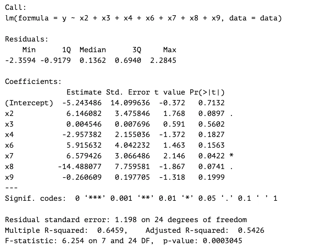
model <- lm(y ~ x2 + x3 + x4 + x6 + x7 + x8 + x9, data = data)

summary(model)

Output:

Analysis and Interpretations

Model Summary

Based on a significance level of $0.05$, all but $x7$ ’s p-value obtained from the values of the t-statistic are greater than $0.05$ which means that the predictors, individually, do not have a relationship with the response variable $y$. Predictor $x7$ has the lowest p-value of $0.0422$, less than $0.05$, which means that there is a relationship between $y$ and $x7$. $x7$ is a statistically significant predictor of $y$. When interpreting the F-statistic, the overall p-value of the model is $0.0003045$, which is less than $0.05$.

Further analysis

This means that the seven predictors in the model do have a relationship with the response variable $y$ and the overall model is statistically significant. Based on both the multiple R-squared and adjusted R-squared values, it can be concluded that many data points are close to the linear regression function line. Both R-squared values are greater than $0.5$ which means that the relationship of the model and the response variable is quite strong. More than $50$ $$% of the variance in the response variable is collectively explained by the predictors.

Quantile-Quantile Plot

Based on the quantile-quantile plot, both the two sets of quantiles (residuals and theoretical quantiles) came from the same distribution since the data points form a line that is roughly straight in a 45 degrees angle. A conclusion that can be drawn from the quantile-quantile plot is that the residuals of our model are normally distributed.

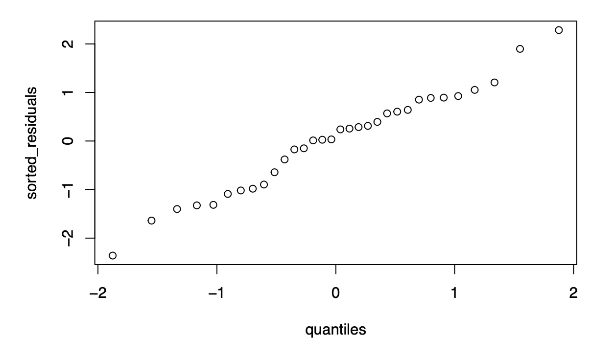
Used qnorm and plot to create qq plot

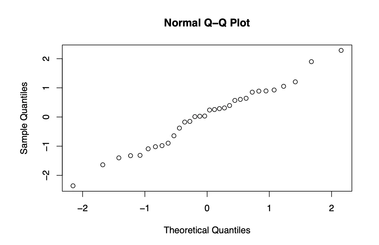
Used qqnorm to create qq plot

R-squared, Adjusted R-squared, and F-statistic

The model has an R-squared value of $0.6459$, which is greater than $50$%; therefore, it can be concluded that the linear model fits the data well since roughly $64$% of the variance found in the response variable can be explained by the seven predictors chosen. The adjusted R-squared value is noticeably lower than the R-squared value. Since R-squared will always increase as more predictors are included in the model and it assumes that all the predictors affect the result of the model, the adjusted R-squared is the preferred measure for this model.

Further analysis

The approximately $10$% difference between the R-squared value and the adjusted R-squared value suggests that not all of the predictors actually have an effect on the performance of the model. The model can be optimized to include only the predictors that affect the model. The F-statistic of the model is $6.254$, which is far from $1$, with a p-value of $0.0003045$. This indicates a relationship between the response variable and the predictors.

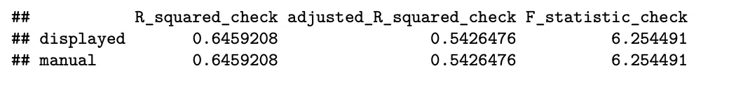
Displayed values are from summary(model) and manual values are manually calculated

Manual Model Reduction

Step 1

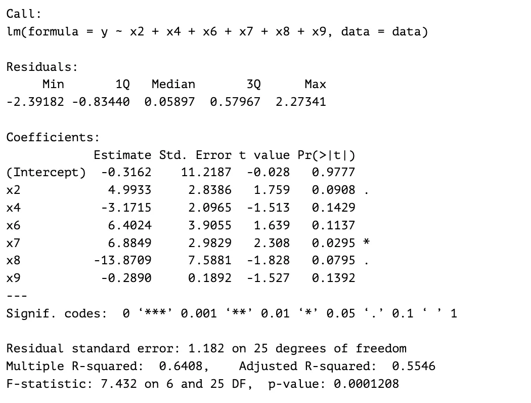
I decided to eliminate predictor $x3$ due to its p-value and coefficient estimate. The p-value is $0.5602$, meaning that $x3$ does not have a statistically significant relationship with the response variable $y$. The coefficient estimate value is near $0$; therefore, the effect of predictor $x3$ to $y$ is small. The resulting model has a smaller overall model p-value at $0.000128$ and the residual standard error has decreased as well.

Output:

Step 2

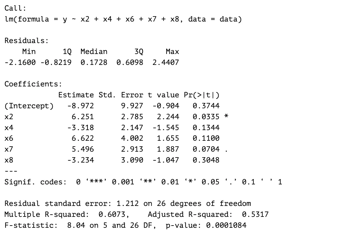
The second predictor eliminated is $x9$. This predictor is eliminated due to the p-value and coefficient estimate. The two predictors with the largest p-values are $x4$ and $x9$, but $x9$ is eliminated first because its coefficient estimate is closer to $0$ than $x4$’s coefficient estimate. This means that $x9$’s effect on the response variable is smaller than $x4$. The resulting model has a smaller overall p-value and a larger F-statistic value, but the R-squared and adjusted R-squared values have decreased.

Output:

Step 3

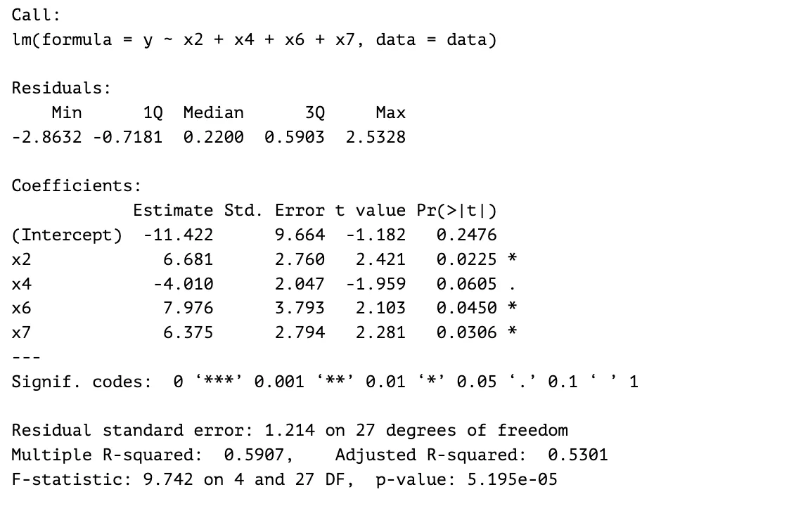
The next predictor eliminated is $x8$. The p-value is one of the reasons why it’s eliminated. It has a p-value of $0.3048$, which is significantly larger than the p-values of the other predictors. Its coefficient estimate is closest to $0$ in comparison to the other predictors which means that it has the least effect on the response variable. The resulting model has a larger F-statistic value and a smaller overall p-value. The adjusted R-squared value was somewhat preserved. The previous model’s adjusted R-squared value is $0.5317$, while the current model’s adjusted R-squared value is $0.5301$.

Output:

Step 4

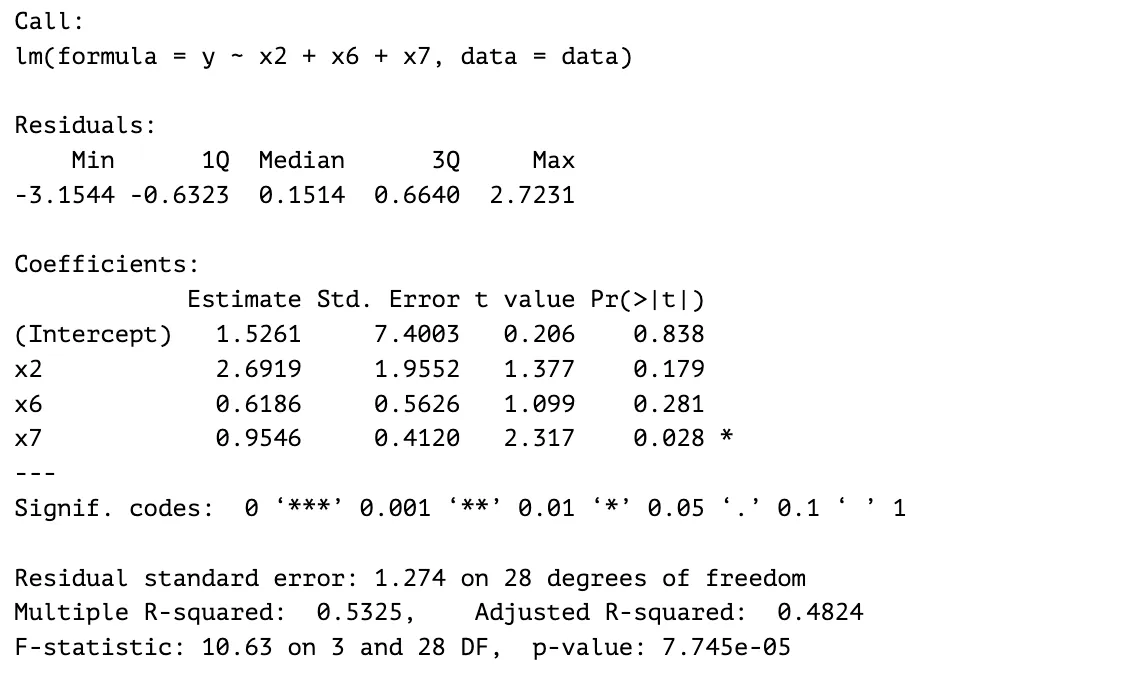
The predictor with the least significance for the model, $x4$, is eliminated. Its p-value is $0.0605$, the largest p-value out of the four predictors. I tried different combinations of three predictors out of the four predictors from the previous model. The three-predictor model with the highest adjusted R-squared after the experiment is the model with predictors $x2$, $x6$, and $x7$. It has a larger F-statistic value, lower overall p-value and lower residual standard error; therefore, $x4$ is eliminated.

Output:

Step 5

The last predictor eliminated in this process is $x6$, which has the largest p-value and a coefficient estimate closer to $0$. These values indicate that $x6$ is the least significant predictor out of the three predictors. The resulting model has a larger F-statistic value and overall p-value, while its adjusted R-squared value has decreased by $0.0037$. From these results, $x2$ and $x7$ seem to be significant predictors to the response variable since the adjusted R-squared value did not have decrease drastically.

Output:

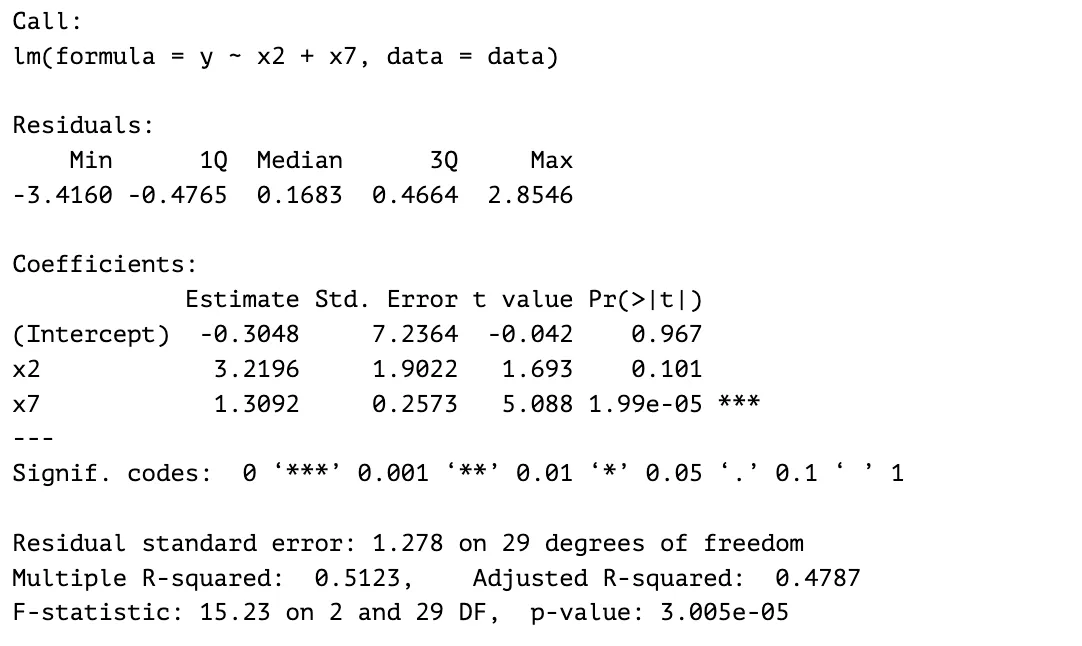
Seven-predictor Model v.s. Two-predictor Model: R-squared interpretation

The seven-predictor model has a larger R-squared and adjusted R-squared values compared to the two-predictor model. The seven-predictor model fits the data better than the two-predictor model. Roughly $47.87$% of the variations in $y$ is explained by $x2$ and $x7$ in the two-predictor model, while $54.26$% of the variations in $y$ is explained by the seven predictors in the seven-predictor model. On the other hand, the two-predictor model has a higher F-statistic value that is further from $1$. It is an indicator that there is a relationship between the predictors and the response variable in the two-predictor model. Based on the R-squared and adjusted R-squared values, the seven-predictor model fits the data better, but the F-statistic value suggests that the two-predictor model is the more significant model.

Results

• Seven-predictor model
  • R-squared: $0.6459208$
  • Adjusted R-squared: $0.5426476$
  • F-statistic: $6.254491$
• Two-predictor model
  • R-squared: $0.5123325$
  • Adjusted R-squared: $0.4787002$
  • F-statistic: $15.233373$

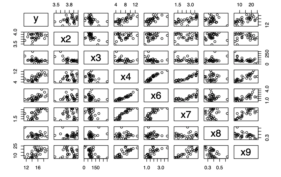
Scatterplot Matrix Analysis

The two predictors chosen in the two-predictor model are $x2$ and $x7$. Based on the scatterplot matrix below, the decision of choosing $x7$ as one of the predictors is supported since the scatterplot matrix shows a more linear relationship between $y$ and $x7$ when compared to the other predictors. As for $x2$, the scatterplot matrix does not show a linear relationship between $y$ and $x2$. The scatterplot matrix somewhat supports my conclusions from the manual model reduction.

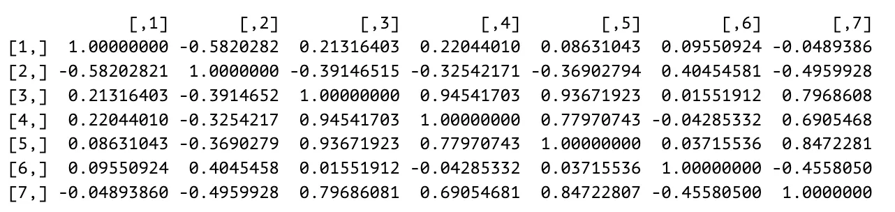
Correlation Matrix Analysis

Since collinearity can be indicated by two variables with a correlation coefficient that is close to $1.0$ and multicollinearity is present when several independent variables in a model are correlated, based on the correlation matrix $W^TW$, there are indications of multicollinearity in the model. There are two pairs of independent variables that are collinear. $W^TW[4,3]$ and $W^TW[3,4]$ have a correlation coefficient of $0.94541703$, showing a positive relationship between the independent variables $x_4$ and $x_6$ as well as collinearity. The same can be said about $W^TW[3,5]$ $W^TW[5,3]$ whose correlation coefficient is $0.93671923$, indicating a positive relationship and collinearity between the independent variables $x_4$ and $x_7$. Since several independent variables in the model are correlated, multicollinearity is indicated in the model.

Variance Inflation Factors Analysis

Based on the variance inflation factors calculated, there are evidence of multicollinearity. $x4$, $x6$, $x7$, $x8$, and $x9$ have high VIF values, which means that they can be predicted by other independent variables in the model, indicating high multicollinearity between each of these independent variables and others. $x2$ and $x3$ VIF values are between $1$ and $5$, indicating moderate multicollinearity.

##         x2         x3         x4         x6         x7         x8         x9
##   3.834363   3.482089 543.612369 158.543426 163.111339   7.355703  27.849239

Condition Indices

Condition indices can be used as indicators of multicollinearity and based on the “MPV” textbook, the numbers to look out for are $100-1000$, indicating moderate to severe multicollinearity, and numbers over $1000$, indicating strong multicollinearity. Out of the condition indices displayed below, the last two numbers stand out, $191.100000$ and $3822.000000$. Based on the benchmarks given in the textbook, there seems to be either a moderate or strong multicollinearity. When the condition number is examined, it can be concluded that the data shows strong multicollinearity, since this number is $3822.000000$.

## [1]    1.000000    2.722222    2.983607   11.375000   28.102941  191.100000
## [7] 3822.000000

Plot of Standardized Residuals v.s. Fitted Values

The plot of standardized residuals against the fitted values for the young wines data does not exhibit any strong unusual pattern. There seems to be a slight tendency for the model to under-predict lower wine quality. The first data point on the left could be a potential outlier since it is the only data point in the lower end of the fitted value that has a residual value of $-2$, but this has to be explored to confirm or deny the assumption.

Further analysis

The residuals for fitted values that fall in the 14 to 16 range has a wider spread, approximately $-2$ to $1$, but most of the data points are randomly scattered around the zero horizontal line, not showing any strong unusual patterns. The data points with fitted values greater than $16$ seem to be scattered around the zero horizontal line. There are two noticeable data points that has residuals of approximately $2$ and fitted values of approximately $17$, that may be potential outliers. These data points are noticeably far from the rest of the data points at that range of fitted values. This idea has to be explored.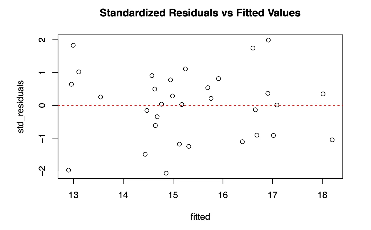

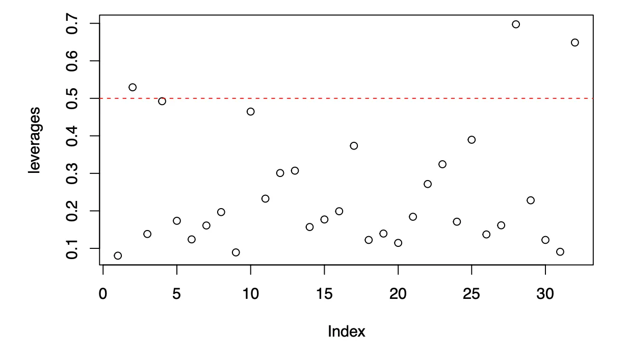
Plot of Leverages

Large leverages reveal observations that are potentially influential because they are remote in $x$ space from the rest of the sample. When looking at the scatter plot of the leverages against the indices from $1$ to $32$, I used the traditional assumption that any observation for which the leverage exceeds twice the average ($2p/n$) is remote enough from the rest of the data to potentially be influential on the regression coefficients. I added a horizontal line with the value $2p/n$, which is $0.5$, in the plot to help detect any influential observations. Based on the plot, observations $2$, $28$, and $32$ exceed twice the average. Out of the three observations, only observations $28$ and $32$ are influential because observation $2$ lies almost on the line passing through the remaining observations. I would investigate observations $28$ and $32$ further to understand why they have a significant impact on the model.

Conclusion

This statistical analysis assignment on youngwines.txt data, focusing on linear regression models, has significantly enhanced my understanding of interpreting regression results. Through the examination of statistics, including p-values, t-statistics, and F-statistics, I gained an increased comprehension of the individual predictors’ impact on wine quality. The manual model reduction process further sharpened my ability to discern the significance of each predictor, refining my grasp of variable selection. The analysis of diagnostic plots, such as quantile-quantile and standardized residuals, provided practical insights into model performance and potential outliers. Overall, this hands-on experience has improved my proficiency in interpreting linear regression outcomes and deepened my understanding of the broader applications of statistical analysis.